import torchAt the heart of how almost every modern machine learning model learns is a process called gradient descent. The core idea is to minimize a “loss” function, which is a score that tells us how wrong our model’s predictions are.
Calculating the gradients for complex models used to involve pages of manual calculus. This is where PyTorch’s autograd engine comes in—it automatically computes these gradients for us, forming the backbone of deep learning. Let’s see how it works with a simple example.
We’ll start with a random guess for the weight w and use gradient descent to guide it toward the true value of 2.
# We want to find a 'w' such that y is close to w * x.
# The true 'w' is clearly 2.
X = torch.tensor([1.0, 2.0, 3.0, 4.0], dtype=torch.float32)
Y = torch.tensor([2.0, 4.0, 6.0, 8.0], dtype=torch.float32)

# Initialize our weight 'w' with a random guess.
# requires_grad=True tells PyTorch to track this tensor for gradient calculations.
w = torch.tensor(0.0, dtype=torch.float32, requires_grad=True)
The key here is requires_grad=True. This tag the w tensor, telling PyTorch’s autograd engine to keep track of every operation involving it so it can later compute gradients.
def forward(x):
    return w * x

def loss(y, y_predicted):
    return ((y_predicted - y)**2).mean()

learning_rate = 0.01
n_iters = 20
print(f"Starting training... Initial weight w = {w.item():.3f}")
weights_history = []
loss_history = []
for epoch in range(n_iters):
    # Forward pass
    y_pred = forward(X)

    # loss
    l = loss(Y, y_pred)
    weights_history.append(w.item())
    loss_history.append(l.item())

    # Calculate gradients = backward pass
    # core of autograd. It calculates the derivative of 'l'
    # with respect to every tensor that has requires_grad=True (i.e., 'w').
    l.backward() # dl/dw

    # Manually update weights
    # torch.no_grad() because this is not part of the computation graph
    with torch.no_grad():
        # The calculated gradient is now in w.grad
        # Update rule: w = w - learning_rate * gradient
        w.data -= learning_rate * w.grad

    # Zero out the gradients for the next iteration
    if (epoch + 1) % 2 == 0:
        print(f'Epoch {epoch+1}: w = {w.item():.3f}, w gradient: {w.grad}, loss = {l.item():.8f}')

    w.grad.zero_()

    # if (epoch + 1) % 2 == 0:
    #     print(f'Epoch {epoch+1}: w = {w.item():.3f}, w gradient: {w.grad}, loss = {l.item():.8f}')

print(f"\nTraining finished. The learned weight is: {w.item():.3f}")
print("The true weight was 2.0")
Starting training... Initial weight w = 0.000
Epoch 2: w = 0.555, w gradient: -25.5, loss = 21.67499924
Epoch 4: w = 0.956, w gradient: -18.423751831054688, loss = 11.31448650
Epoch 6: w = 1.246, w gradient: -13.311159133911133, loss = 5.90623236
Epoch 8: w = 1.455, w gradient: -9.61731243133545, loss = 3.08308983
Epoch 10: w = 1.606, w gradient: -6.948507308959961, loss = 1.60939169
Epoch 12: w = 1.716, w gradient: -5.020296096801758, loss = 0.84011245
Epoch 14: w = 1.794, w gradient: -3.627163887023926, loss = 0.43854395
Epoch 16: w = 1.851, w gradient: -2.6206254959106445, loss = 0.22892261
Epoch 18: w = 1.893, w gradient: -1.8934016227722168, loss = 0.11949898
Epoch 20: w = 1.922, w gradient: -1.3679819107055664, loss = 0.06237914
Training finished. The learned weight is: 1.922
The true weight was 2.0The plots below show the loss steadily decreasing while the weight w converges towards its target value.
import matplotlib.pyplot as plt

# Create the plots
fig = plt.figsize=(8, 10)

# Plot 1: Loss vs. Epochs
plt.plot(loss_history, 'r-')
plt.title("Loss vs. Epochs")
plt.xlabel("Epoch")
plt.ylabel("Loss")
plt.show()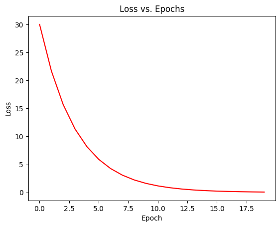
# Create the plots
fig = plt.figsize=(8, 10)

# Plot 2: Weight vs. Epochs
plt.plot(weights_history, 'b-')
plt.axhline(y=2.0, color='g', linestyle='--', label="True Weight") # Add line for the true weight
plt.title("Weight (w) vs. Epochs")
plt.xlabel("Epoch")
plt.ylabel("Weight (w)")
plt.legend()
plt.show()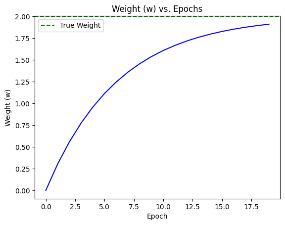
While our example was simple, these exact principles: defining a model, calculating loss, and using autograd to update parameters, power the training of massive neural networks.